4 Results

4.1 Model Output

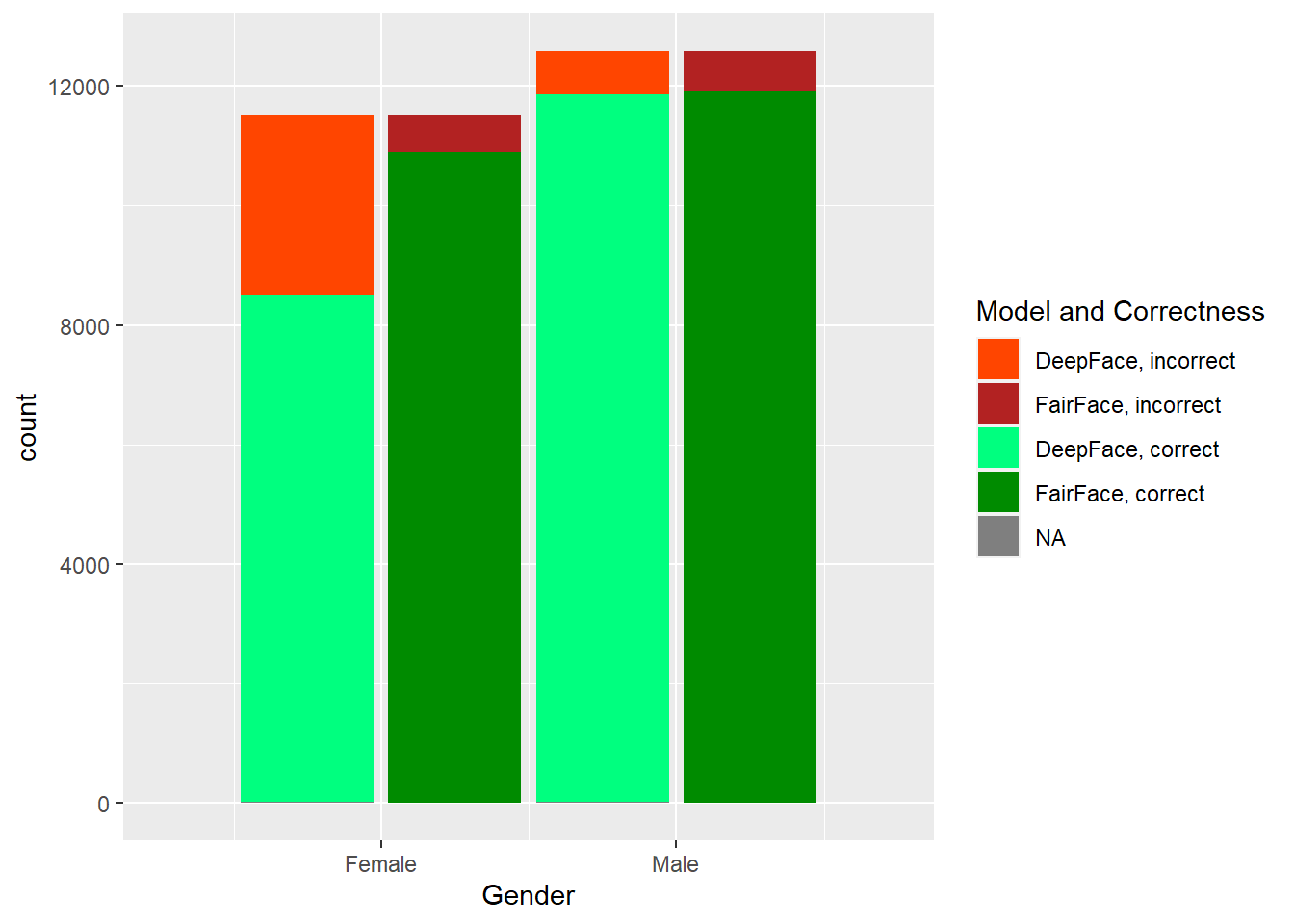
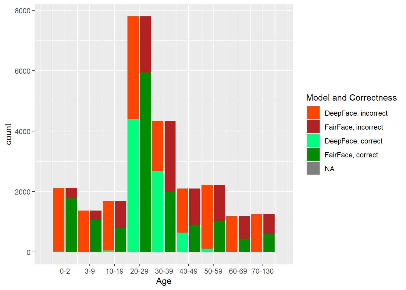
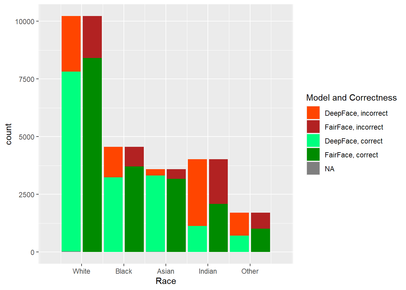
The two models, DeepFace and FairFace, were run on the dataset described previously. In Figure 4.1, one can see the results of the predictions done by each model, by each factor that was considered: age, gender, and race. Note that the total (across correct and incorrect) histogram distributions match the correct (source dataset) distributions of values in each category, so we can see exactly the difference between what was provided and what was predicted, along with how well each model did on each category within each factor.

4.2 Model Performance, Hypothesis Testing

For each factor category and model, we calculate the F1 score, accuracy, p-value, and power, as described in section 3. Cell values are colored according to the strength of the metric; p-value is colored as to whether it crosses the significance value threshold of 0.003. We calculate these metrics and hypothesis tests across all categories of each factor, but also with conditional filtering on other factors; the value “All” indicates we did not filter/condition on that factor. The column Test Factor indicates which factor we are calculating the proportion for that hypothesis test. For example, the following column value subsets would indicate the given hypothesis test:

Test Factor	Age	Gender	Race	Model	Null Hypothesis	Description
gender	0-2	Female	All	FairFace	\(p_{F, D_f \| A_1} = p_{F,D_0 \| A_1}\)	\(H_0\) : The proportions of Female labels, given that the source age label is 0-2, are equal.
race	All	All	Black	DeepFace	\(p_{R_B, D_d} = p_{R_B, D_0}\)	\(H_0\): The proportions of Black labels are equal.

The results are summarized in Table 4.1, which is interactive and filterable.

Table 4.1: Table of F1 score, accuracy, p-value, and power, by each factor and category evaluated by the models, with a potential filtering condition.

4.2.1 p-value Critical Values

From the previous table, we extract and highlight key values; namely, where we reject the null hypothesis and where we do not, based on our criteria:

Significance level of 99.7%
Power threshold of 0.8
F1-Score of 0.9

Disclaimer - we are not claiming that F1-scores and and p-values are directly tied to one another, but exploring its use here as a means by which we can more confidently reject the null hypothesis.

Which come from the rationale described in Chapter 3. We show the test values where there is no sub-filtering/conditions by another category; then, we also highlight the reverse null hypothesis decisions made with filtering for a sub-condition and for the specific rows as described in the table captions. The values are displayed in Table 4.2. There is only a Fairface table for not rejecting the null hypothesis (with no condition subfiltering) because no DeepFace values passed our given thresholds for not rejecting; the same reasoning is why there is no table for FairFace rejecting the null hypothesis with condition subfiltering.

Table 4.2: Highlighted statistics/metrics for DeepFace and FairFace, that pass the given significance level/power/F1-score thresholding.

(a) FairFace: Reject the null hypothesis, with no condition subfiltering

	Category	p-Value	Power	F1 Score
age	70-130	2.83e−43	1.0000	0.6271
	3-9	1.37e−05	0.9198	0.7176
	10-19	5.22e−05	0.8640	0.5052
	0-2	3.11e−06	0.9568	0.8960
	20-29	2.14e−08	0.9959	0.7333
	40-49	1.65e−08	0.9965	0.3944
race	White	5.83e−18	1.0000	0.8610
	Black	7.46e−12	1.0000	0.8685
	Indian	8.84e−94	1.0000	0.6402
	Other	0.00e00	1.0000	0.3087

(b) FairFace: Do not reject the null hypothesis, for the factor category given in (a), for subcondition filtering

	Age	Gender	Race	p-Value	Power	F1 Score
age	0-2	Male	All	4.94e−01	0.0120	0.9190

	Category	p-Value	Power	F1 Score
age	70-130	1.08e−283	1.0000	NA
	3-9	9.20e−293	1.0000	NA
	10-19	2.52e−148	1.0000	0.0479
	0-2	0.00e00	1.0000	NA
	20-29	2.00e−65	1.0000	0.5054
	30-39	0.00e00	1.0000	0.3786
	40-49	1.65e−91	1.0000	0.2276
	50-59	3.66e−202	1.0000	0.0802
	60-69	9.81e−229	1.0000	0.0016
gender	Female	1.18e−97	1.0000	0.8198
gender	Male	1.18e−97	1.0000	0.8637
race	White	2.70e−27	1.0000	0.8095
	Asian	1.75e−143	1.0000	0.7039
	Black	1.71e−33	1.0000	0.7965
	Indian	1.90e−292	1.0000	0.4092
	Other	4.64e−262	1.0000	0.2389

(d) DeepFace: Do not reject the null hypothesis, for the factor category given in (c), for subcondition filtering

	Age	Gender	Race	p-Value	Power	F1 Score
gender	30-39	Male	All	7.70e−02	0.1185	0.9224

(e) FairFace: Do not reject the null hypothesis, with no condition subfiltering

	Category	p-Value	Power	F1 Score
gender	Female	7.07e−01	0.0053	0.9429
gender	Male	7.07e−01	0.0053	0.9476

4.3 Meta-Analysis Plots

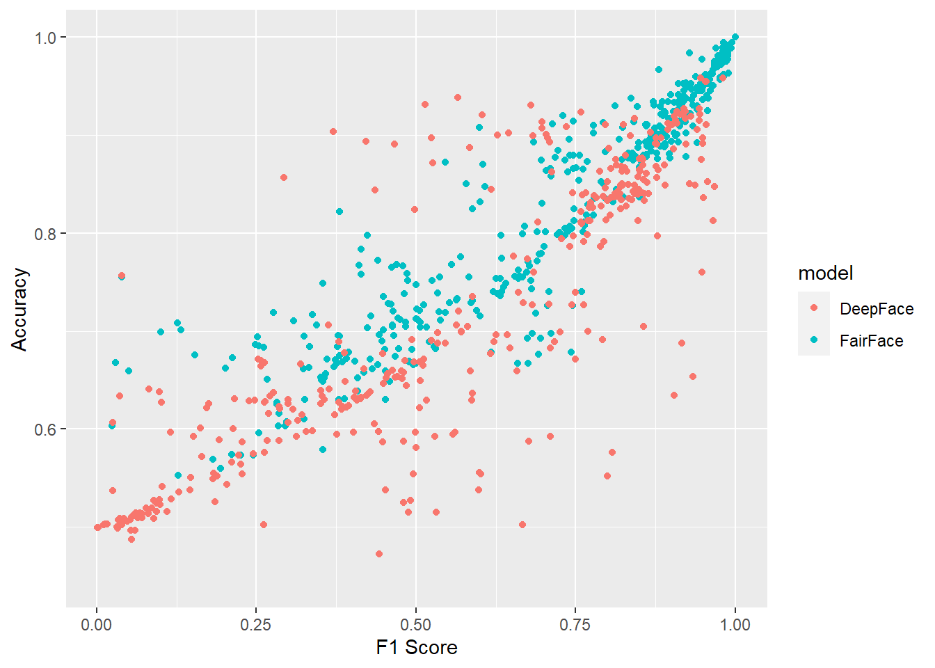
In Figure 4.2, we show F1-score vs accuracy for all hypothesis tests that were performed. Note the relationship is not perfectly linear.

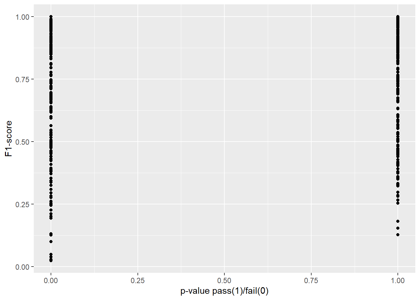
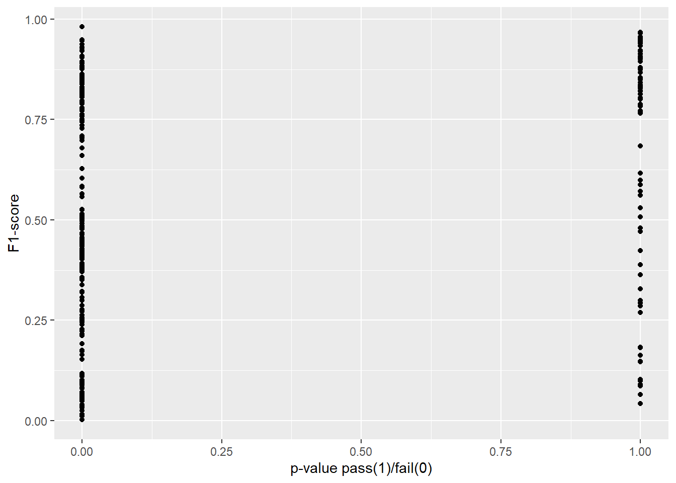
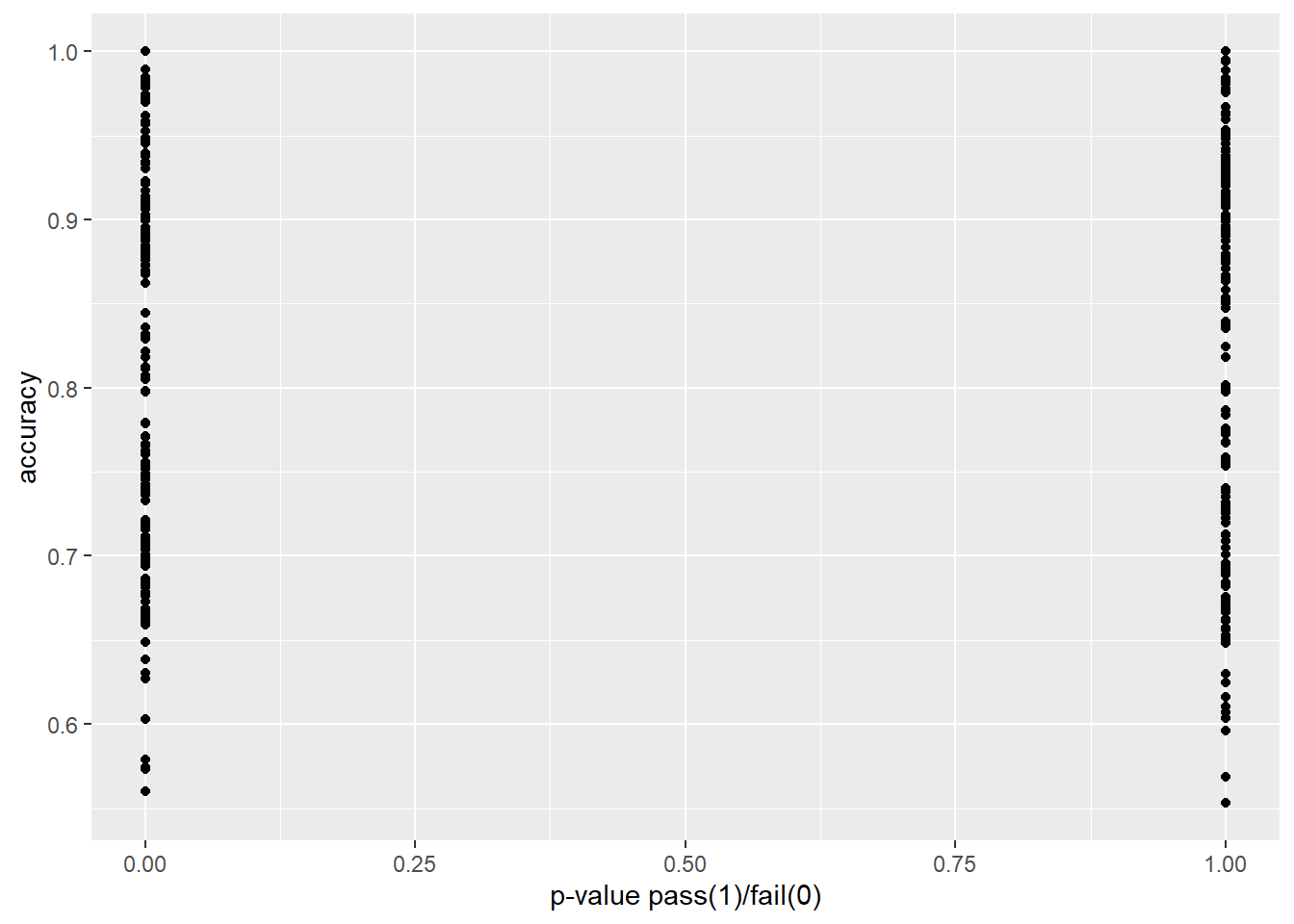
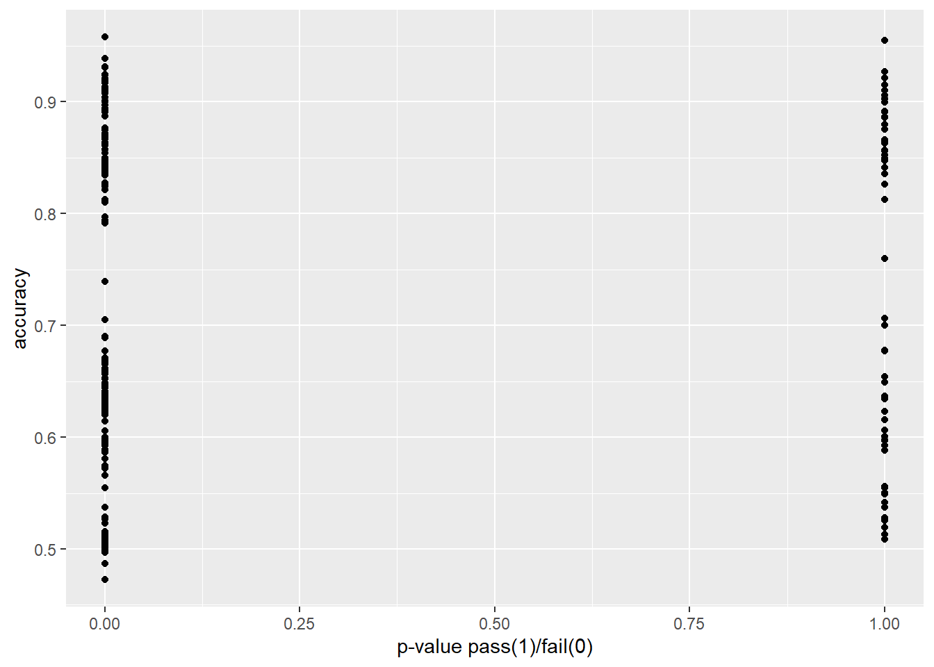
Figure 4.2: F1-Score vs Accuracy for all hypothesis tests performed.

In Figure 4.3 and Figure 4.4 we explore our research question of whether or not two-sample proportion tests can approximate or predict the performance of a machine learning model. In each plot, we transform the p-value to 0 in cases where we would reject the null hypothesis, and 1 in cases for which we would fail to reject.

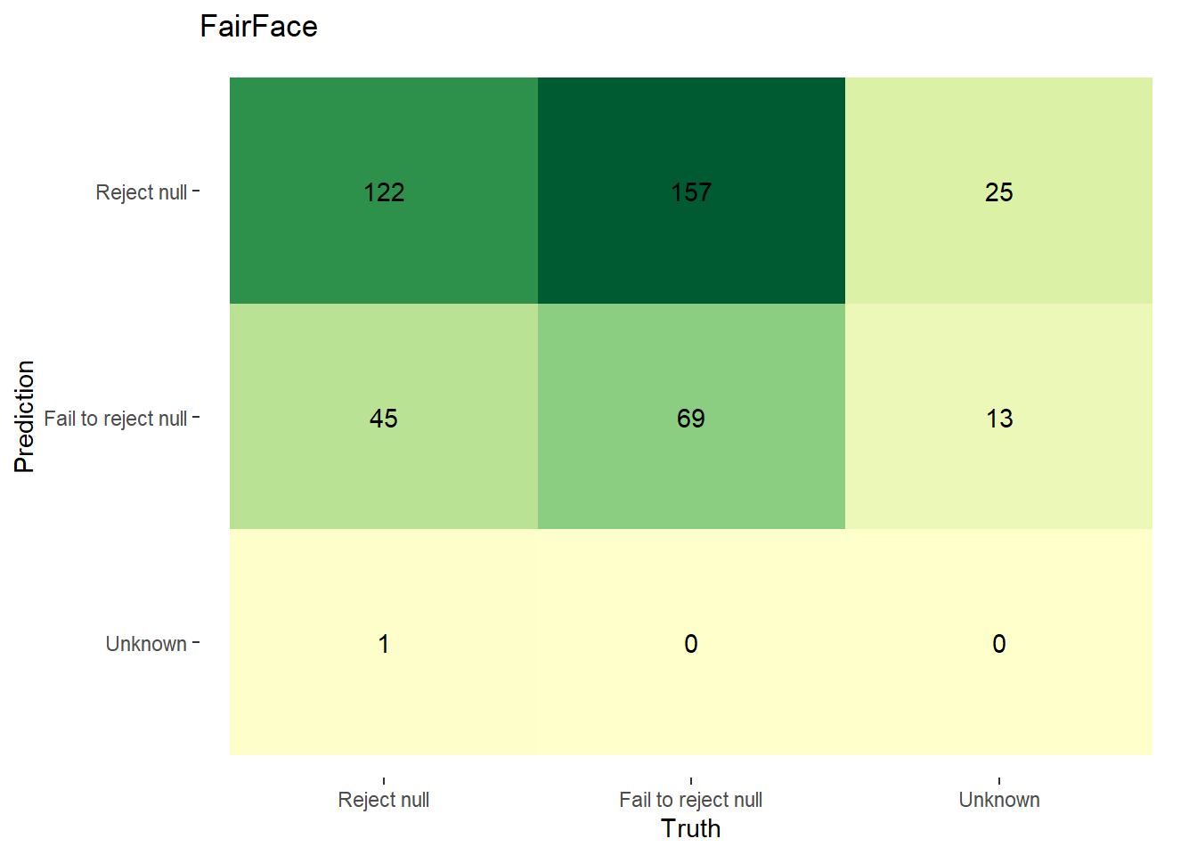
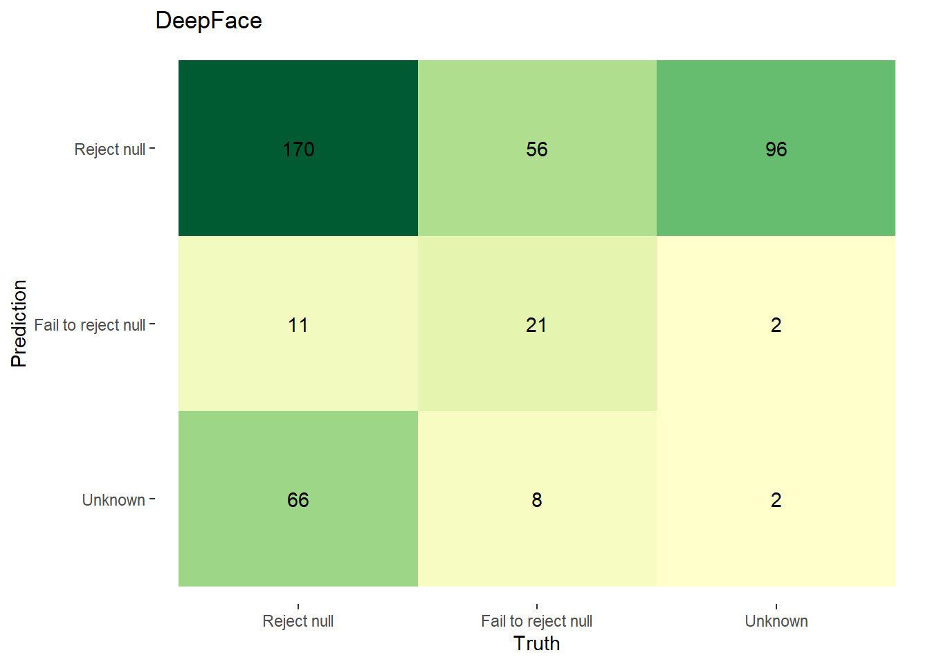
(a) FairFace: two-sample proportion p-value vs F1

(a) FairFace: two-sample proportion p-value vs accuracy

In Figure 4.5, we display confusion matrices of our null hypothesis rejections. We define the true/false positive/negatives as follows:

Predicted Classification	Actual Classification	Classification
p-value < 0.003 & pwr >= 0.8	F1 < 0.9	Reject Null
p-value >= 0.003	F1 >= 0.9	Fail to Reject Null
p-value < 0.003 & pwr < 0.8; pval is NA; pwr is NA	F1 is NA	Unknown/Further Inspection Needed

Using the above, the confusion matrices for FairFace and DeepFace are as follows:

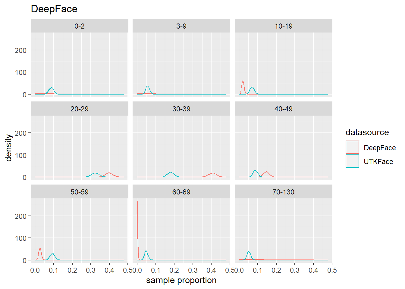
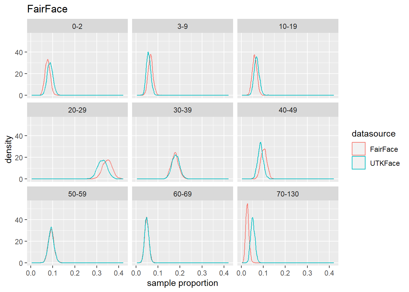
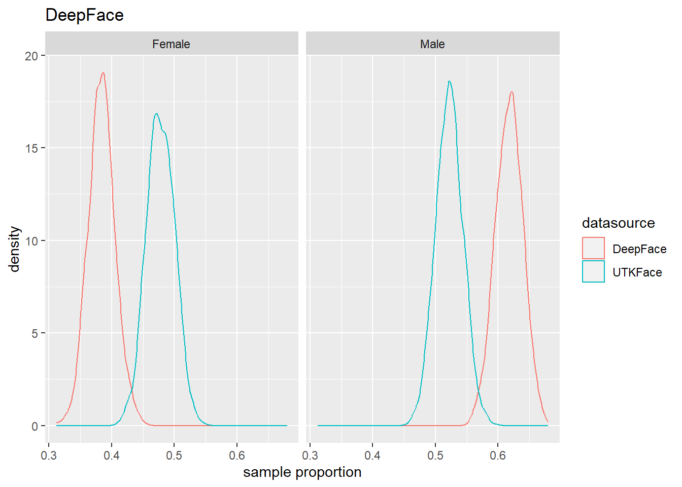
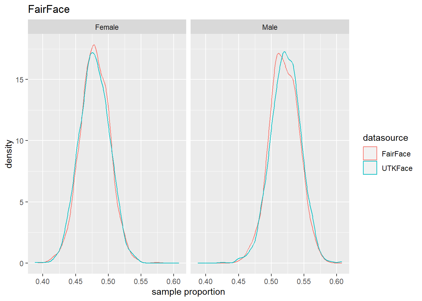
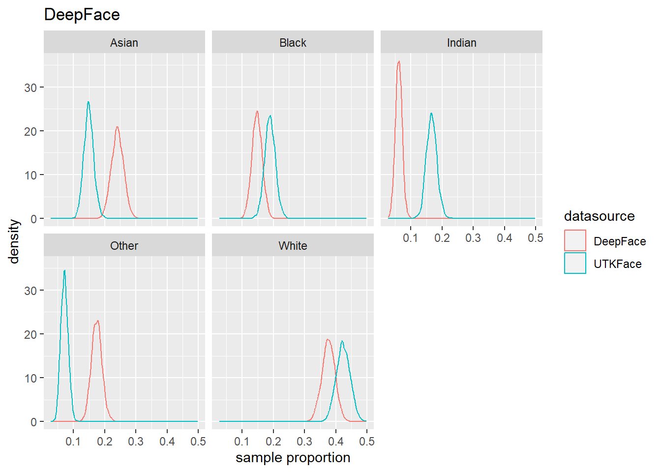
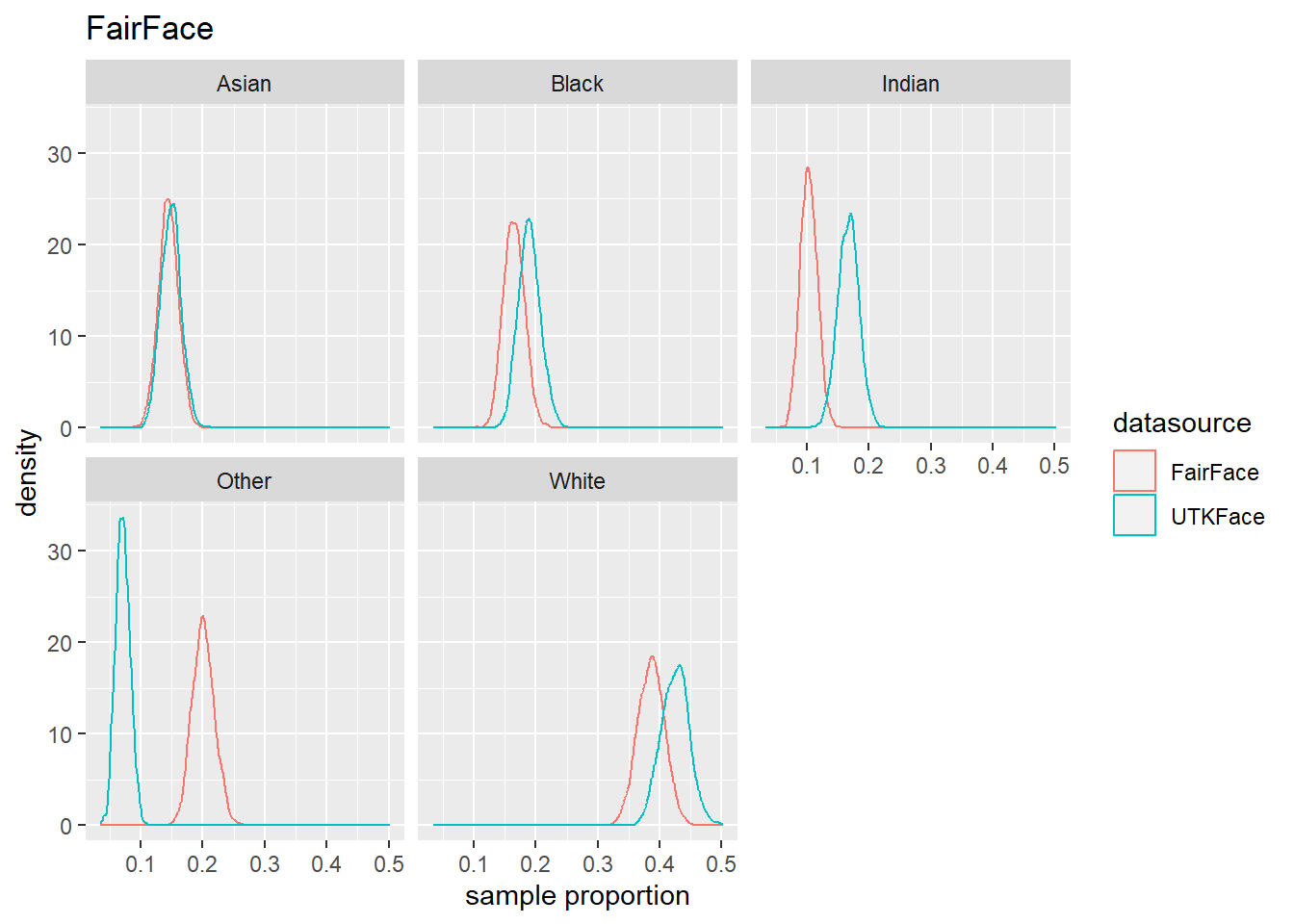
4.4 Population Estmate Plots - UTK Face vs. Model

We used a resampling technique to produce estimated population proportion distributions for each sample. Each resampling included 2000 samples of 500 subjects under their respective test conditions.

To support our analysis and conclusions, we leveraged a resampling technique (bootstrap sampling) to build approximations of each sample’s parent population. The resampling took 2000 samples of 500 random subjects, with replacement, to build the estimated distribution of proportions in the population under specified test conditions. The plots can be seen in Figure 4.6 to Figure 4.8. We find that these plots coincide with our hypothesis testing results – namely, that higher p-values result in greater overlap between the predicted and actual distributions, and lower p-values result in less overlap between the distributions. As such, these distributions will support us in drawing our conclusions.

(a) DeepFace vs. UTKFace Age Distributions

(a) DeepFace vs. UTKFace Gender Distributions

(a) DeepFace vs. UTKFace Race Distributions